1. Preprocessing expression data
This tutorial demonstrate how to pre-process single-cell raw UMI counts to generate expression matrices that can be used as input to cell-cell communication tools. We recommend the quality control chapter in the Single-cell Best Practices book as a starting point for a detailed overview of QC and single-cell RNAseq analysis pipelines in general.
We demonstrate a typical workflow using a SingleCellExperiment object. We recommend using SCE because it is less memory intensive and has better compatiblity with LIANA. However, if you prefer Seurat, we have also provided a supplementary tutorial for preprocessing with that tool
For these tutorials, we will use a lung dataset of 63k immune and epithelial cells across three control, three moderate, and six severe COVID-19 patients.
Details and caveats regarding batch correction, which removes technical variation while preserving biological variation between samples, can be viewed in the Batch Correction Supplementary Tutorial.
Preparare the object for cell-cell communication analysis
Import the required libraries
[1]:
suppressPackageStartupMessages({
    library(scater, quietly = TRUE)
    library(scran, quietly = TRUE)
    library(scuttle, quietly = TRUE)

    library(BiocParallel, quietly = TRUE)
    library(parallel, quietly = TRUE)
#     library(scDblFinder, quietly = TRUE) ## TODO Add to environment.yml

    library(ggplot2, quietly = TRUE)
    library(cowplot, quietly = TRUE)
})

options(timeout=600)
[2]:
# paths
data.path <- file.path("..", "..", "data")
if (!dir.exists(data.path)){
    dir.create(data.path)
}
[3]:
# parallelization
n.cores<-parallel::detectCores() # default to all
if (n.cores<=1){
    bpparam<-BiocParallel::SerialParam()
}else{
    bpparam<-BiocParallel::MulticoreParam(workers = n.cores)
}
Loading
The 12 samples can be downloaded as .h5 files from here. You can also download the cell metadata from here
Alternatively, the SCE Object can be downloaded using this link. See this notebook for how the object was built using the above files.
[4]:
covid_data <- readRDS(url('https://zenodo.org/record/7706962/files/BALF-COVID19-Liao_et_al-NatMed-2020_SCE.rds'))
colData(covid_data)
DataFrame with 63103 rows and 9 columns
                       orig.ident      sample  sample_new     disease
                      <character> <character> <character> <character>
AAACCCACAGCTACAT-1_1         C100        C100         HC3           N
AAACCCATCCACGGGT-1_1         C100        C100         HC3           N
AAACCCATCCCATTCG-1_1         C100        C100         HC3           N
AAACGAACAAACAGGC-1_1         C100        C100         HC3           N
AAACGAAGTCGCACAC-1_1         C100        C100         HC3           N
...                           ...         ...         ...         ...
TTTGTCATCGATAGAA-1_12         C52         C52         HC2           N
TTTGTCATCGGAAATA-1_12         C52         C52         HC2           N
TTTGTCATCGGTCCGA-1_12         C52         C52         HC2           N
TTTGTCATCTCACATT-1_12         C52         C52         HC2           N
TTTGTCATCTCCAACC-1_12         C52         C52         HC2           N
                          hasnCoV   cluster   cell.type   condition    ident
                      <character> <integer> <character> <character> <factor>
AAACCCACAGCTACAT-1_1            N        27           B     Control     C100
AAACCCATCCACGGGT-1_1            N        23 Macrophages     Control     C100
AAACCCATCCCATTCG-1_1            N         6           T     Control     C100
AAACGAACAAACAGGC-1_1            N        10 Macrophages     Control     C100
AAACGAAGTCGCACAC-1_1            N        10 Macrophages     Control     C100
...                           ...       ...         ...         ...      ...
TTTGTCATCGATAGAA-1_12           N         2 Macrophages     Control      C52
TTTGTCATCGGAAATA-1_12           N         3 Macrophages     Control      C52
TTTGTCATCGGTCCGA-1_12           N         2 Macrophages     Control      C52
TTTGTCATCTCACATT-1_12           N         3 Macrophages     Control      C52
TTTGTCATCTCCAACC-1_12           N         2 Macrophages     Control      C52
Calculate Basic QC metrics
We will calculate some basic QC metrics associated with the library size that will be used for filtering:
[5]:
covid_data <- scater::addPerCellQC(covid_data)
Quality-Control Filtering
Exclude cells that visually do not fall within the normal range of standard QC metrics (see chapter) – fraction of genes in a cell that are mitochondrial, number of unique genes, and total number of genes measured.
[6]:
min.features <- 200
min.cells <- 3

sce_counts <- counts(covid_data)

if (min.features > 0) {
  nfeatures <- Matrix::colSums(x = sce_counts > 0)
  sce_counts <- sce_counts[, which(x = nfeatures >= min.features)]
}
# filter genes on the number of cells expressing
if (min.cells > 0) {
  num.cells <- Matrix::rowSums(x = sce_counts > 0)
  sce_counts <- sce_counts[which(x = num.cells >= min.cells), ]
}

covid_data<-covid_data[rownames(sce_counts), colnames(sce_counts)]
Get the fraction of genes that are mitochondrial:
[7]:
is.mito <- grep("MT-", rownames(covid_data))
per.cell <- scuttle::perCellQCMetrics(covid_data, subsets=list(Mito=is.mito))
colData(covid_data)[['subsets_Mito_percent']] <- per.cell$subsets_Mito_percent
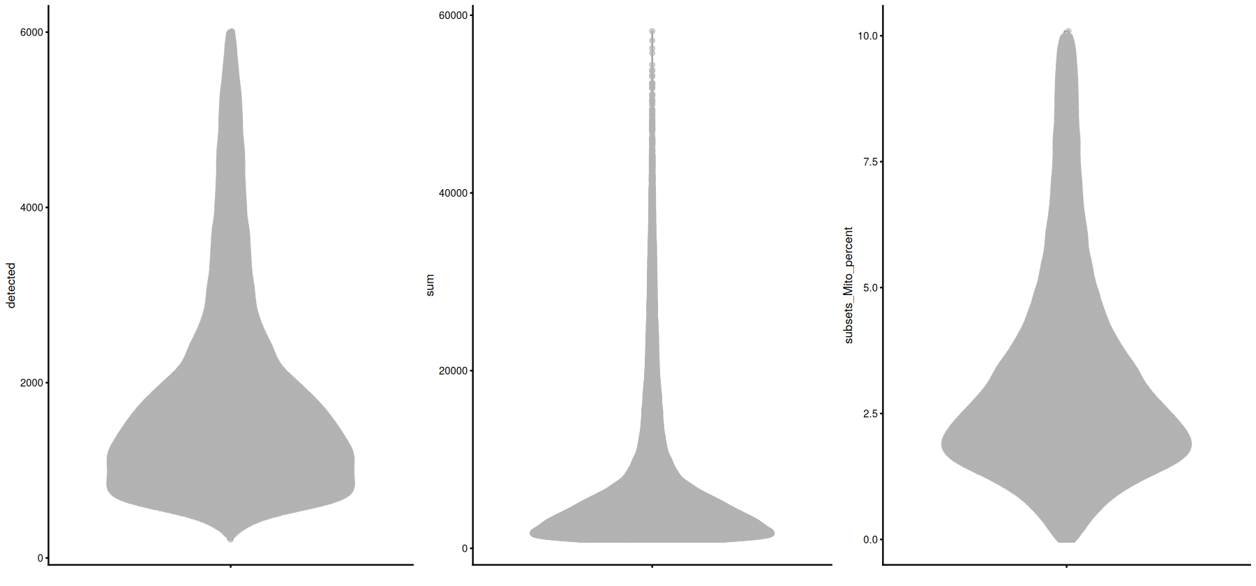
From left to right, plot the total unique features, the total counts, and the fraction of mitochondrial genes in each cell:
[8]:
h_ = 7
w_ = 15
options(repr.plot.height=h_, repr.plot.width=w_)

g1A <- scater::plotColData(object = covid_data, y = 'detected')
g1B <- scater::plotColData(object = covid_data, y = 'sum')
g1C <- scater::plotColData(object = covid_data, y = 'subsets_Mito_percent')
g1 <- cowplot::plot_grid(g1A, g1B, g1C, ncol = 3)

g1
[9]:
md <- data.frame(covid_data@colData)

g2A <- ggplot(data = md, aes(x = sum, y = subsets_Mito_percent)) + geom_point(size = 0.5)
g2B <- ggplot(data = md, aes(x = sum, y = detected)) + geom_point(size = 0.5)
g2 <- cowplot::plot_grid(g2A, g2B, ncol = 2)
g2
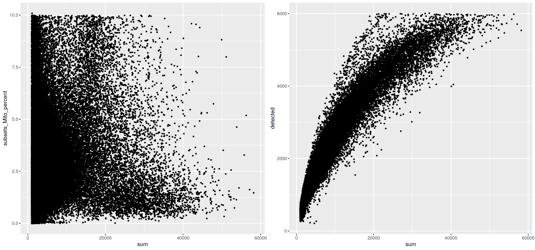
We can remove any droplets with high mitochondrial content or those that potentially represent doublets:
[10]:
covid_data <- covid_data[, colData(covid_data)$subsets_Mito_percent < 15]
covid_data <- covid_data[, colData(covid_data)$detected < 5500]
Note that in this case we filter out cells with high total counts, but a best practice approach would be to instead filter out doublets. As using different doublet detection techniques in R and Python introduces some differences between the workflows, we will not do this here.
Nevertheless, the code for doublet detection is provided below:
set.seed(100)
covid_data <- scDblFinder(covid_data, samples="sample_new")
Normalize
For single-cell inference across sample and across cell types, most CCC tools require the library sizes to be comparable. We can use the scuttle function normalizeCounts to log- and library-normalize the counts. This function divides each cell by the total counts per cell and multiplies by the median of the total counts per cell. Furthermore, we log1p-transform the data to make it more Gaussian-like, as this is a common assumption for the analyses downstream. Finally, such a normalization
maintains non-negative counts, which is important for tensor decomposition.
[11]:
scale.factor <- 1e4
lib.sizes <- colSums(counts(covid_data)) / scale.factor
assay(covid_data, 'logcounts') <- scuttle::normalizeCounts(covid_data, size.factors=lib.sizes, log=FALSE, center.size.factors=FALSE)
assay(covid_data, 'logcounts') <- log1p(assay(covid_data, 'logcounts'))
Dimensionality Reduction
While dimensionality reduction is not used directly in these tutorials, a number of these steps are necessary to obtain cell group labels when processing your own data. Steps such as filtering for highly variable genes (HVGs) and scaling the data improve dimensionality reudction and clustering results. However, for CCC, we recommend using the entire gene expression matrix unscaled (either raw or library- and log-normalized). Scaling introduces negative counts, which poses challenges for CCC inference or tensor decompsoition. Filtering for HVGs reduces the list of potential ligand-receptor pairs that can be tested for interactions.
This tutorial diverges with its companion tutorial in Python here due to minor algorithmic differences, but since the inputs will be the full expression matrices above, these discrepancies will not affect downstream tutorials.
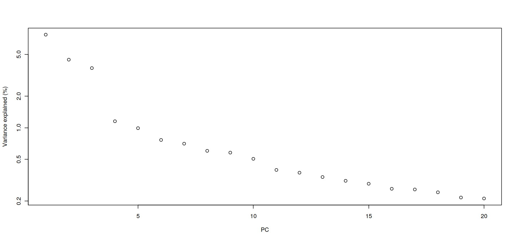
[12]:
# hvgs<-scran::getTopHVGs(covid_data, n = 2000)

covid_data <- scater::runPCA(covid_data,
                             exprs_values = "logcounts",
                             scale = TRUE,
                             ntop = 2000,
                             ncomponents = 20,
                             BPPARAM = bpparam
                            )

percent.var <- attr(reducedDim(covid_data), "percentVar")
plot(percent.var, log="y", xlab="PC", ylab="Variance explained (%)")
Warning message in selectChildren(jobs, timeout):
“error 'No child processes' in select”
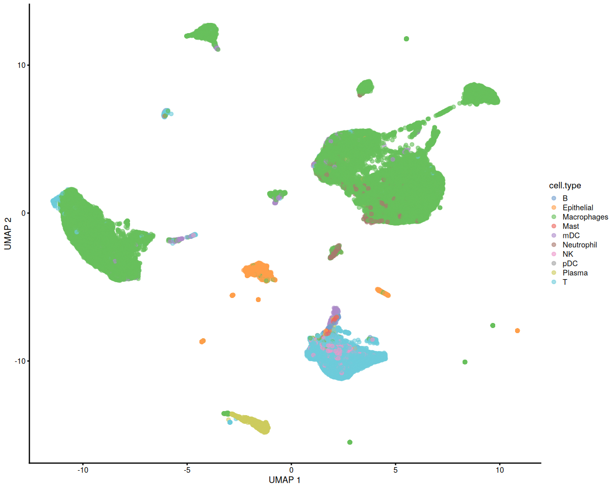
[13]:
h_ = 8
w_ = 10
options(repr.plot.height=h_, repr.plot.width=w_)

n.pcs<-20
# scran::buildSNNGraph(covid_data, use.dimred = 'PCA', d = n.pcs, )


covid_data <- scater::runUMAP(covid_data,
                              pca = n.pcs,
                              dimred = 'PCA',
                              BPPARAM = bpparam
                             )
scater::plotUMAP(covid_data, colour_by = 'cell.type')
[14]:
saveRDS(covid_data, file.path(data.path, 'covid_balf_norm.rds'))