S4. Identify CCC patterns from spatial transcriptomics

This tutorial illustrates how LIANA and Tensor-cell2cell can be used to explore cell-cell communication in distinct regions of a tissue using spatial transcriptomics. Here each region of the tissue is treated as a separate context.

Initial Setups

Enabling GPU use

First, if you are using a NVIDIA GPU with CUDA cores, set use_gpu=True and enable PyTorch with the following code block. Otherwise, set use_gpu=False or skip this part

use_gpu = True

if use_gpu:
    import tensorly as tl
    tl.set_backend('pytorch')

Libraries

Then, import all the packages we will use in this tutorial:

import cell2cell as c2c
import decoupler as dc
import liana as li

import numpy as np
import pandas as pd
import scanpy as sc
import squidpy as sq

import matplotlib.pyplot as plt
import seaborn as sns

from scipy.spatial.distance import squareform

import warnings
warnings.filterwarnings('ignore')

Directories

Afterwards, specify the data and output directories:

output_folder = '../../data/spatial/'
c2c.io.directories.create_directory(output_folder)

../../data/spatial/ was created successfully.

Load data

Similar to the tutorial of using LIANA and MISTy, we will use an ischemic 10X Visium spatial slide from Kuppe et al., 2022. It is a tissue sample obtained from a patient with myocardial infarction, specifically focusing on the ischemic zone of the heart tissue.

The slide provides spatially-resolved information about the cellular composition and gene expression patterns within the tissue.

adata = sc.read("kuppe_heart19.h5ad", backup_url='https://figshare.com/ndownloader/files/41501073?private_link=4744950f8768d5c8f68c')

adata

AnnData object with n_obs × n_vars = 4113 × 17703
    obs: 'in_tissue', 'array_row', 'array_col', 'sample', 'n_genes_by_counts', 'log1p_n_genes_by_counts', 'total_counts', 'log1p_total_counts', 'pct_counts_in_top_50_genes', 'pct_counts_in_top_100_genes', 'pct_counts_in_top_200_genes', 'pct_counts_in_top_500_genes', 'mt_frac', 'celltype_niche', 'molecular_niche'
    var: 'gene_ids', 'feature_types', 'genome', 'SYMBOL', 'n_cells_by_counts', 'mean_counts', 'log1p_mean_counts', 'pct_dropout_by_counts', 'total_counts', 'log1p_total_counts', 'mt', 'rps', 'mrp', 'rpl', 'duplicated'
    uns: 'spatial'
    obsm: 'compositions', 'mt', 'spatial'

Process data

Normalize data

adata.layers['counts'] = adata.X.copy()
sc.pp.normalize_total(adata, target_sum=1e4)
sc.pp.log1p(adata)

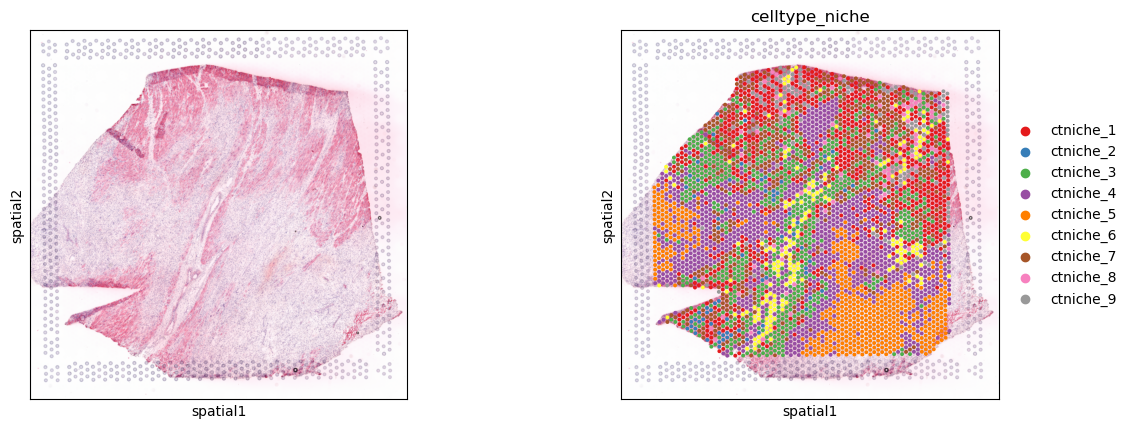
Visualize spot clusters or niches. These niches were defined by clustering spots from their cellular composition deconvoluted by using cell2location (Kuppe et al., 2022).

sq.pl.spatial_scatter(adata, color=[None, 'celltype_niche'], size=1.3, palette='Set1')

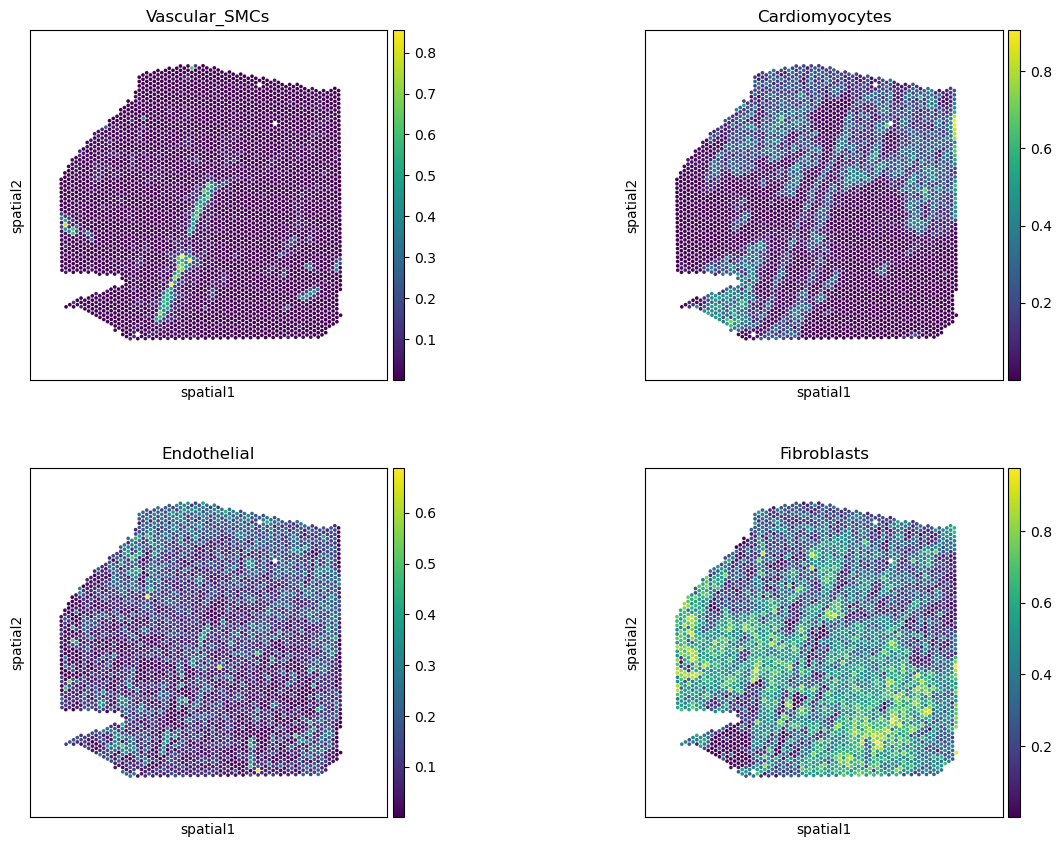
Cellular composition obtained from cell2location

# Rename to more informative names
full_names = {'Adipo': 'Adipocytes',
              'CM': 'Cardiomyocytes',
              'Endo': 'Endothelial',
              'Fib': 'Fibroblasts',
              'PC': 'Pericytes',
              'prolif': 'Proliferating',
              'vSMCs': 'Vascular_SMCs',
              }
# but only for the ones that are in the data
adata.obsm['compositions'].columns = [full_names.get(c, c) for c in adata.obsm['compositions'].columns]

comps = li.ut.obsm_to_adata(adata, 'compositions')

comps.var

Adipocytes
Cardiomyocytes
Endothelial
Fibroblasts
Lymphoid
Mast
Myeloid
Neuronal
Pericytes
Proliferating
Vascular_SMCs

# check key cell types
sq.pl.spatial_scatter(comps,
                      color=['Vascular_SMCs','Cardiomyocytes',
                             'Endothelial', 'Fibroblasts'],
                      size=1.3, ncols=2, img_alpha=0
                      )

adata_og = adata.copy()

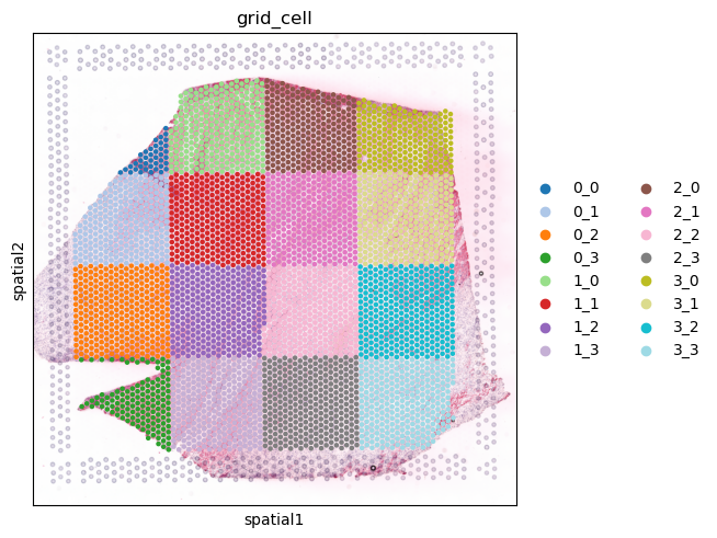
Defining spatial contexts in the tissue

For defining spatial contexts within a tissue using spatial transcriptomics we simply divide the tissue in different regions through a square grid of a specific number of bins in each of the axes.

In this case, we divide our tissue into a 4x4 grid. A new column will be create in the adata object, specifically adata.obs['grid_cell'], to assign each spot or cell a grid window.

num_bins = 4

c2c.spatial.create_spatial_grid(adata, num_bins=num_bins)

sq.pl.spatial_scatter(adata, color='grid_cell', size=1.3, palette='tab20')

... storing 'grid_cell' as categorical

Here, cells or spots in one grid window do not get to interact with those that are within other grid windows, ignoring that cells in the interfaces between grid windows could also interact. For accounting for those cases, more complex approaches could be employed, as for example a sliding window strategy for defining contexts. In that case, spatial contexts will present some overlap in the cells or spots that are within them.

For simplicity we only tried the grid approach, which could be replaced by the sliding windows method, but it would also require to account for the overlap between spatial contexts. If you are interested in trying out this approach, see cell2cell.spatial.neighborhood.create_sliding_windows() and cell2cell.spatial.neighborhood.add_sliding_window_info_to_adata().

Deciphering cell-cell communication

Here we run LIANA to compute interactions between spots or cells aggregated by their corresponding cluster/niche annotations. Interactions are computed for each spatial context (grid window) by considering only cells annotated with such spatial context in the grid_cell column in the adata.obs DataFrame.

In this case we use the CellPhoneDB list of ligand-receptor interactions, and the CellPhoneDB method to infer CCC.

cell_group = 'celltype_niche'

lr_pairs = li.resource.select_resource('cellchatdb')

li.mt.cellphonedb.by_sample(adata, resource=lr_pairs, groupby=cell_group, sample_key='grid_cell',
                            expr_prop=0.1, use_raw=False, verbose=True)

Now running: 3_3: 100%|█████████████████████████| 16/16 [01:16<00:00,  4.78s/it]

The results are located here:

spatial_liana = adata.uns['liana_res']

spatial_liana

	grid_cell	ligand	ligand_complex	ligand_means	ligand_props	receptor	receptor_complex	receptor_means	receptor_props	source	target	lr_means	cellphone_pvals
0	0_0	FN1	FN1	4.556507	1.000000	ITGAV	ITGAV_ITGB1	2.021336	1.00	ctniche_1	ctniche_3	3.288921	0.083
1	0_0	FN1	FN1	4.556507	1.000000	ITGAV	ITGAV_ITGB1	1.928708	1.00	ctniche_1	ctniche_7	3.242608	0.155
2	0_0	FN1	FN1	4.342961	1.000000	ITGAV	ITGAV_ITGB1	2.021336	1.00	ctniche_3	ctniche_3	3.182149	0.299
3	0_0	FN1	FN1	4.312120	1.000000	ITGAV	ITGAV_ITGB1	2.021336	1.00	ctniche_7	ctniche_3	3.166728	0.374
4	0_0	FN1	FN1	4.342961	1.000000	ITGAV	ITGAV_ITGB1	1.928708	1.00	ctniche_3	ctniche_7	3.135835	0.499
...	...	...	...	...	...	...	...	...	...	...	...	...	...
195553	3_3	WNT3	WNT3	0.064199	0.200000	LRP6	FZD6_LRP6	0.081630	0.20	ctniche_3	ctniche_3	0.072915	0.538
195554	3_3	WNT3	WNT3	0.064199	0.200000	LRP6	FZD1_LRP6	0.081630	0.20	ctniche_3	ctniche_3	0.072915	0.538
195555	3_3	WNT3	WNT3	0.064199	0.200000	LRP6	FZD8_LRP6	0.081630	0.20	ctniche_3	ctniche_3	0.072915	0.538
195556	3_3	POMC	POMC	0.052017	0.104478	MC1R	MC1R	0.078427	0.11	ctniche_4	ctniche_5	0.065222	0.644
195557	3_3	SEMA3A	SEMA3A	0.064199	0.200000	PLXNA4	NRP1_PLXNA4	0.064199	0.20	ctniche_3	ctniche_3	0.064199	0.116

195558 rows × 13 columns

Using LIANA results to build a 4D-communication tensor, with grid windows as the contexts in the 4th dimension.

tensor = li.multi.to_tensor_c2c(liana_res=spatial_liana, # LIANA's dataframe containing results
                                sample_key='grid_cell', # Column name of the samples
                                source_key='source', # Column name of the sender cells
                                target_key='target', # Column name of the receiver cells
                                ligand_key='ligand_complex', # Column name of the ligands
                                receptor_key='receptor_complex', # Column name of the receptors
                                score_key='lr_means', # Column name of the communication scores to use
                                inverse_fun=None, # Transformation function
                                how='outer', # What to include across all samples
                                outer_fraction=1/4., # Fraction of samples as threshold to include cells and LR pairs.
                               )

100%|███████████████████████████████████████████| 16/16 [00:19<00:00,  1.21s/it]

Metadata for coloring the elements in the tensor.

Here we do not assign major groups, each element is colored separately.

dimensions_dict = [None, None, None, None]
meta_tensor = c2c.tensor.generate_tensor_metadata(interaction_tensor=tensor,
                                                  metadata_dicts=dimensions_dict,
                                                  fill_with_order_elements=True
                                                 )

Tensor properties

tensor.shape

torch.Size([16, 700, 9, 9])

tensor.excluded_value_fraction()

0.7867879122495651

tensor.sparsity_fraction()

0.0

Run Tensor-cell2cell pipeline

For simplicity, we factorize the tensor into 8 factors or CCC patterns instead of using the elbow analysis to determine the number of factors.

c2c.analysis.run_tensor_cell2cell_pipeline(tensor,
                                           meta_tensor,
                                           rank=8, # Number of factors to perform the factorization. If None, it is automatically determined by an elbow analysis
                                           tf_optimization='regular', # To define how robust we want the analysis to be.
                                           random_state=0, # Random seed for reproducibility
                                           device='cuda', # Device to use. If using GPU and PyTorch, use 'cuda'. For CPU use 'cpu'
                                           cmaps=['plasma', 'Dark2_r', 'Set1', 'Set1'],
                                           output_folder=output_folder, # Whether to save the figures in files. If so, a folder pathname must be passed
                                          )

Running Tensor Factorization
Generating Outputs
Loadings of the tensor factorization were successfully saved into ../../data/spatial//Loadings.xlsx

<cell2cell.tensor.tensor.PreBuiltTensor at 0x7f9a75deb3d0>

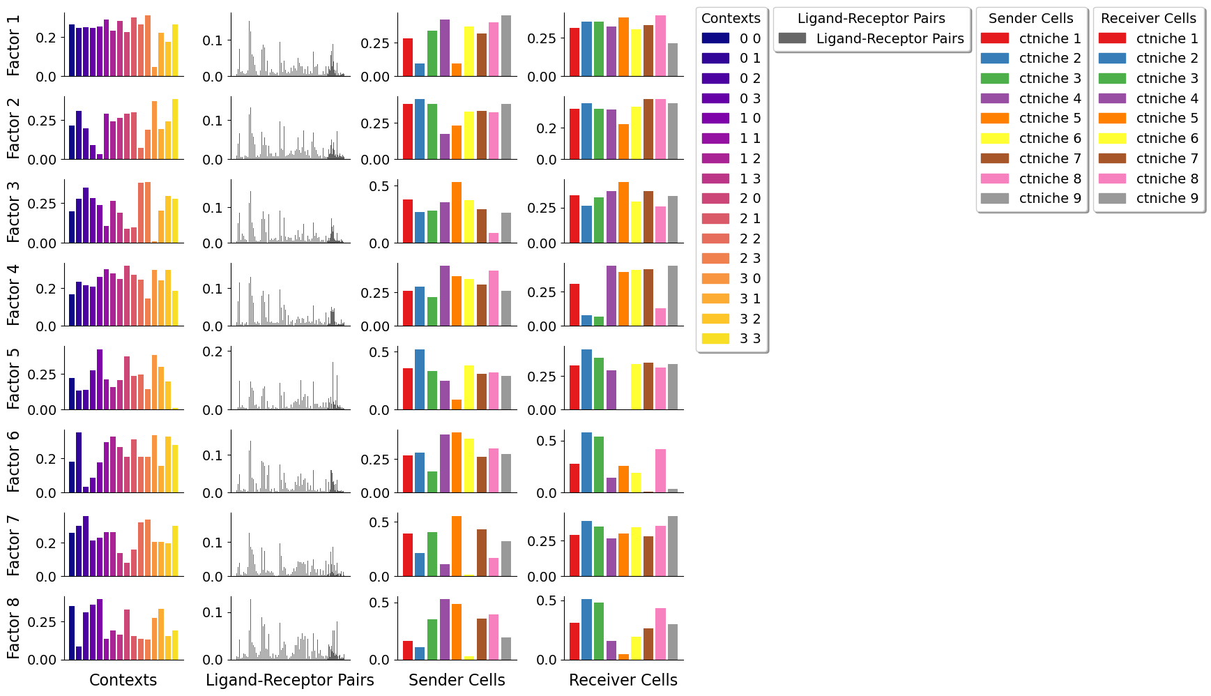
Visualize CCC patterns in space

Each factor or CCC pattern contains loadings for the context dimension. These loadings could be mapped for each spot or cell depending on what spatial context (grid window) they belong to. Thus, we can visualize the importance of each context in each of the factors, and see how the CCC patterns behave in space.

This behavior in space is useful to understand what set of LR pairs are used by determinant sender-receiver spot pairs in each region of the tissue. Regions with higher scores, indicate that LR pairs of that factor are used more there by the senders and receivers with high loadings.

# Generate columns in the adata.obs dataframe with the loading values of each factor
factor_names = list(tensor.factors['Contexts'].columns)
for f in factor_names:
    adata.obs[f] = adata.obs['grid_cell'].apply(lambda x: float(tensor.factors['Contexts'][f].to_dict()[x]))
    adata.obs[f] = pd.to_numeric(adata.obs[f])

# These columns are used for coloring the tissue regions to associate them with each factor
sq.pl.spatial_scatter(adata, color=[None, 'celltype_niche']+factor_names, size=1.3, cmap='Blues', vmin=0.)
plt.suptitle(f'{num_bins}x{num_bins} Spatial Grid', fontsize=32, ha='left')

Text(0.5, 0.98, '4x4 Spatial Grid')

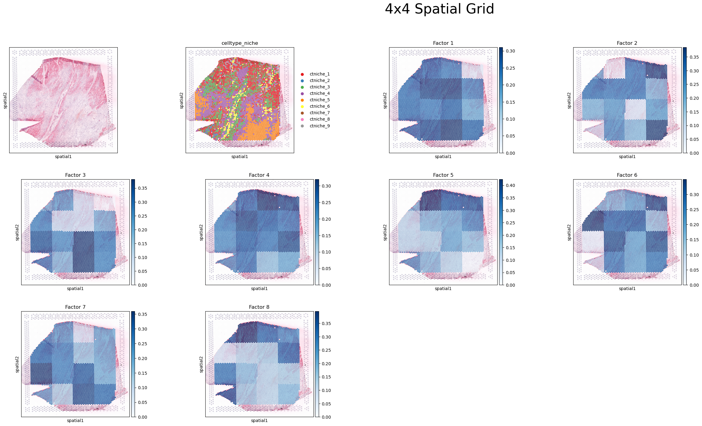
For example, we can take Factor 5 here, and see that regions in the top area of the tissue, and the bottom left corner are associated with the CCC pattern. Here, main interacting spots are niches 1 and 2 (mainly composed of cardiomyocytes and endothelial cells), coinciding with the areas where they are mainly located.

Then, using the LR pair loadings, we can also identify LR interactions that are key in each factor, and link this with the spatial region with higher scores in the same factor.

_ = c2c.plotting.loading_clustermap(loadings=tensor.factors['Ligand-Receptor Pairs'],
                                    loading_threshold=0.1,
                                    use_zscore=False,
                                    figsize=(28, 8),
                                    filename=None,
                                    row_cluster=False
                                   )

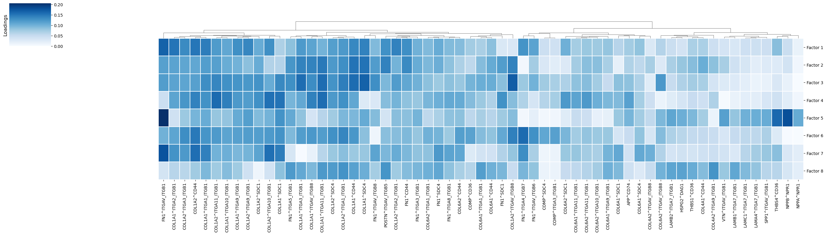
In factor 5, where interactions of niches 1 and 2 are associated with this CCC pattern, LR interactions such as NPPB^NPR1, THBS4^CD36, and FN1^ITGAV&ITGB1 are important.

Following the same idea, other downstream analyses could be performed (e.g., Pathway enrichment analysis, PROGENy analysis, among others - see this notebook), and use the resulting scores to associate them with important tissue regions per factor.

Finally, for comparing tissues from multiple patients, a 4D tensor could be built for the same tissue region across patients. So the 4th dimension would be a tissue region aligned and present across patients.

Different grid sizes

We can also explore changing the number of bins in the grid to see the impact on the analysis. With this we can focus on shorter- or longer-ranges of interactions.

def run_pipeline_per_bins(adata, lr_pairs, cell_group, bin_list, output_folder=None):
    results = {}
    for num_bins in bin_list:
        if output_folder is not None:
            output_folder = output_folder + '/NumBins-{}/'.format(num_bins)
            c2c.io.directories.create_directory(output_folder)

        tmp_result = {}
        adata_ = adata.copy()
        c2c.spatial.create_spatial_grid(adata_, num_bins=num_bins)

        li.mt.cellphonedb.by_sample(adata_, resource=lr_pairs, groupby=cell_group, sample_key='grid_cell',
                                    expr_prop=0.1, use_raw=False, verbose=True)

        spatial_liana = adata_.uns['liana_res']
        tensor = li.multi.to_tensor_c2c(liana_res=spatial_liana, # LIANA's dataframe containing results
                                        sample_key='grid_cell', # Column name of the samples
                                        source_key='source', # Column name of the sender cells
                                        target_key='target', # Column name of the receiver cells
                                        ligand_key='ligand_complex', # Column name of the ligands
                                        receptor_key='receptor_complex', # Column name of the receptors
                                        score_key='lr_means', # Column name of the communication scores to use
                                        inverse_fun=None, # Transformation function
                                        how='outer', # What to include across all samples
                                        outer_fraction=1/4., # Fraction of samples as threshold to include cells and LR pairs.
                                       )

        dimensions_dict = [None, None, None, None]
        meta_tensor = c2c.tensor.generate_tensor_metadata(interaction_tensor=tensor,
                                                          metadata_dicts=dimensions_dict,
                                                          fill_with_order_elements=True
                                                         )

        c2c.analysis.run_tensor_cell2cell_pipeline(tensor,
                                                   meta_tensor,
                                                   rank=8, # Number of factors to perform the factorization. If None, it is automatically determined by an elbow analysis
                                                   tf_optimization='regular', # To define how robust we want the analysis to be.
                                                   random_state=0, # Random seed for reproducibility
                                                   device='cuda', # Device to use. If using GPU and PyTorch, use 'cuda'. For CPU use 'cpu'
                                                   cmaps=['plasma', 'Dark2_r', 'Set1', 'Set1'],
                                                   output_folder=output_folder, # Whether to save the figures in files. If so, a folder pathname must be passed
                                                  )

        # Generate columns in the adata_.obs dataframe with the loading values of each factor
        factor_names = list(tensor.factors['Contexts'].columns)
        for f in factor_names:
            adata_.obs[f] = adata_.obs['grid_cell'].apply(lambda x: float(tensor.factors['Contexts'][f].to_dict()[x]))
            adata_.obs[f] = pd.to_numeric(adata_.obs[f])

        tmp_result['tensor'] = tensor
        tmp_result['tensor_meta'] = meta_tensor
        tmp_result['adata'] = adata_
        results[num_bins] = tmp_result
    return results

results = run_pipeline_per_bins(adata_og, lr_pairs, cell_group, bin_list=[2,3], output_folder=output_folder)

../../data/spatial//NumBins-2/ was created successfully.

Converting `grid_cell` to categorical!
Now running: 1_1: 100%|███████████████████████████| 4/4 [00:28<00:00,  7.17s/it]
100%|█████████████████████████████████████████████| 4/4 [00:06<00:00,  1.66s/it]

Running Tensor Factorization
Generating Outputs
Loadings of the tensor factorization were successfully saved into ../../data/spatial//NumBins-2//Loadings.xlsx

Converting `grid_cell` to categorical!

../../data/spatial//NumBins-2//NumBins-3/ was created successfully.

Now running: 2_2: 100%|███████████████████████████| 9/9 [00:45<00:00,  5.02s/it]
100%|█████████████████████████████████████████████| 9/9 [00:12<00:00,  1.40s/it]

Running Tensor Factorization
Generating Outputs
Loadings of the tensor factorization were successfully saved into ../../data/spatial//NumBins-2//NumBins-3//Loadings.xlsx

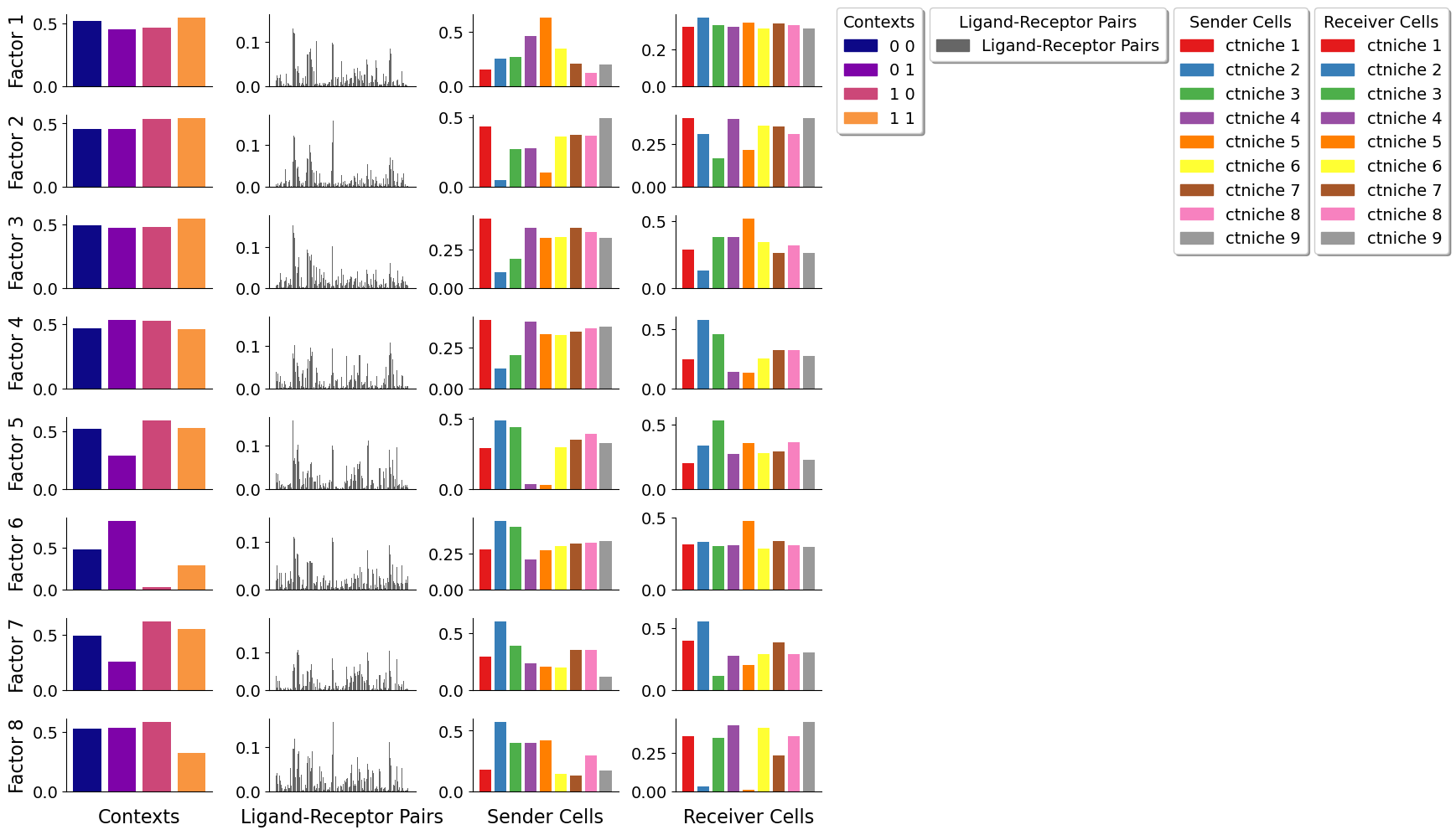
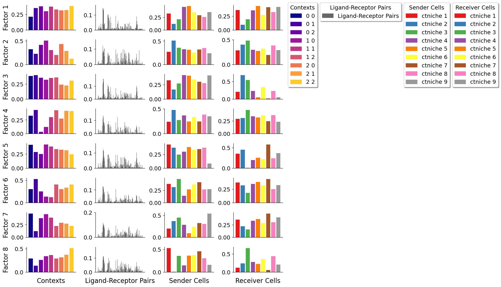
Let’s visualize the imprtant bins per factor for the different grids

for k, v in results.items():
    factor_names = list(v['tensor'].factors['Contexts'].columns)
    sq.pl.spatial_scatter(v['adata'], color=[None, 'celltype_niche']+factor_names, size=1.3, cmap='Blues', vmin=0.)
    plt.suptitle(f'{k}x{k} Spatial Grid', fontsize=32, ha='left')

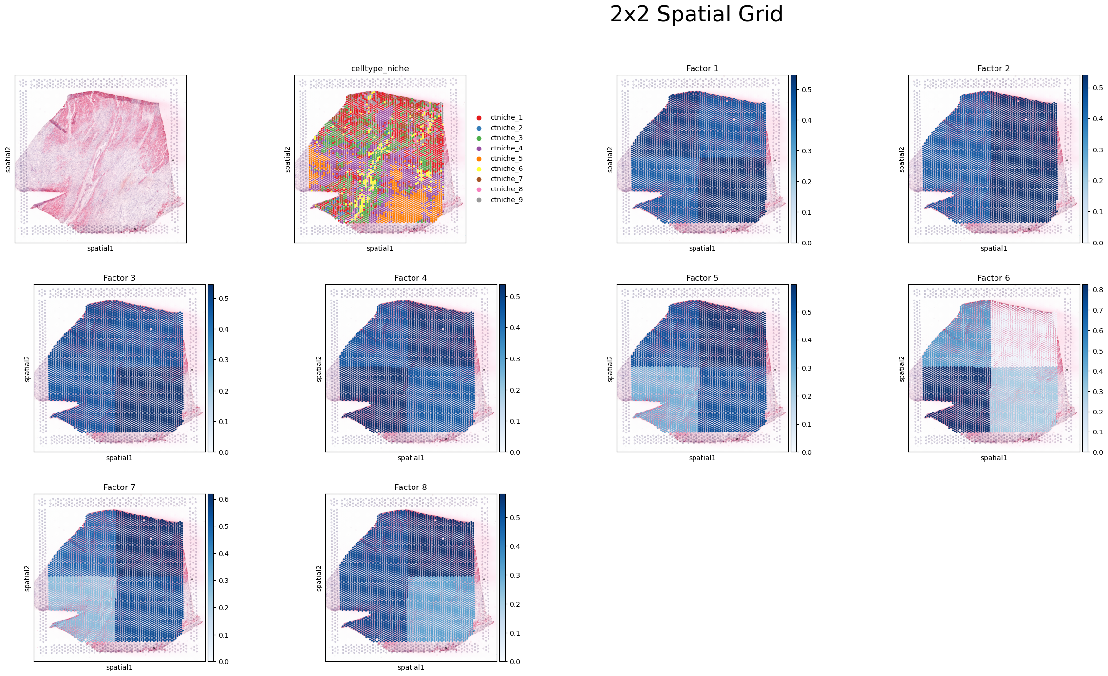
As the size of the grid window increases, it becomes more challenging to discern regional differences within the tissue due to the coarser resolution provided by these larger windows. In this case, more cell-cell interactions are capture per window, making difficult to identify patterns associated with more specific spots. Conversely, smaller grid windows offer a finer resolution, enabling a clearer distinction and more detailed understanding of the variations between different tissue regions.