1. Preprocessing expression data
This tutorial demonstrate how to pre-process single-cell raw UMI counts to generate expression matrices that can be used as input to cell-cell communication tools. We recommend the quality control chapter in the Single-cell Best Practices book as a starting point for a detailed overview of QC and single-cell RNAseq analysis pipelines in general.
We demonstrate a typical workflow using the popular single-cell analysis software scanpy to generate an AnnData object which can be used downstream. For these tutorials, we will use a lung dataset of 63k immune and epithelial cells across three control, three moderate, and six severe COVID-19 patients.
Details and caveats regarding batch correction, which removes technical variation while preserving biological variation between samples, can be viewed in the additional examples tutorial entitled “S1_Batch_Correction”.
Preparare the object for cell-cell communication analysis
Import the required packages
[1]:
import os

import scanpy as sc
import pandas as pd
import numpy as np

import cell2cell as c2c
[2]:
import warnings
warnings.filterwarnings('ignore')
[3]:
data_path = '../../data/'
c2c.io.directories.create_directory(data_path)
../../data/ already exists.
Loading
The 12 samples can be downloaded as .h5 files from here. You can also download the cell metadata from here
Alternatively, cell2cell has a helper function to load the data as an AnnData object:
[4]:
adata = c2c.datasets.balf_covid(os.path.join(data_path, 'BALF-COVID19-Liao_et_al-NatMed-2020.h5ad'))
adata.obs.head()
[4]:
| sample | sample_new | group | disease | hasnCoV | cluster | celltype | condition | |
|---|---|---|---|---|---|---|---|---|
| AAACCCACAGCTACAT_3 | C100 | HC3 | HC | N | N | 27.0 | B | Control |
| AAACCCATCCACGGGT_3 | C100 | HC3 | HC | N | N | 23.0 | Macrophages | Control |
| AAACCCATCCCATTCG_3 | C100 | HC3 | HC | N | N | 6.0 | T | Control |
| AAACGAACAAACAGGC_3 | C100 | HC3 | HC | N | N | 10.0 | Macrophages | Control |
| AAACGAAGTCGCACAC_3 | C100 | HC3 | HC | N | N | 10.0 | Macrophages | Control |
[5]:
adata.obs.condition.unique()
[5]:
['Control', 'Moderate COVID-19', 'Severe COVID-19']
Categories (3, object): ['Control', 'Moderate COVID-19', 'Severe COVID-19']
Calculate Basic QC metrics
We will calculate some basic QC metrics associated with the library size that will be used for filtering:
[6]:
adata.var['mt'] = adata.var_names.str.startswith('MT-')  # annotate the group of mitochondrial genes as 'mt'
sc.pp.calculate_qc_metrics(adata,
                           qc_vars=['mt'],
                           percent_top=None,
                           log1p=False,
                           inplace=True)
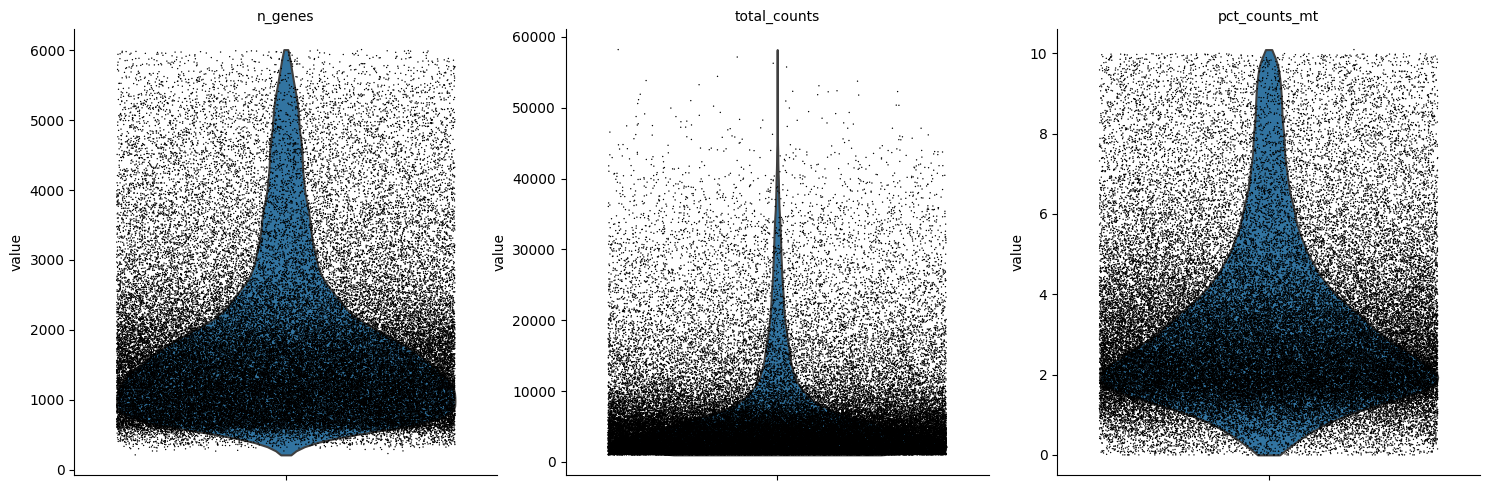
Quality-Control Filtering
Exclude cells that visually do not fall within the normal range of standard QC metrics (see chapter) – fraction of genes in a cell that are mitochondrial, number of unique genes, and potential doublets.
Note that since this is a pre-processed dataset, these steps are largely to demonstrate the workflow.
[7]:
sc.pp.filter_cells(adata, min_genes=200)
sc.pp.filter_genes(adata, min_cells=3)
[8]:
sc.pl.violin(adata, ['n_genes', 'total_counts', 'pct_counts_mt'],
             jitter=0.4, multi_panel=True)
[9]:
sc.pl.scatter(adata, x='total_counts', y='pct_counts_mt')
sc.pl.scatter(adata, x='total_counts', y='n_genes')
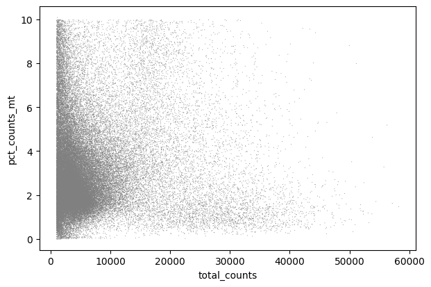
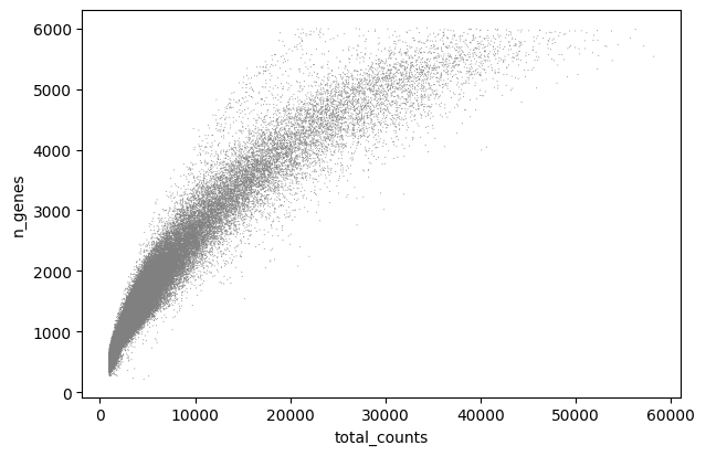
We can remove any droplets with high mitochondrial content or those that potentially represent doublets:
[10]:
adata = adata[adata.obs.pct_counts_mt < 15, :]
adata = adata[adata.obs.n_genes < 5500, :]
Note that in this case we filter out cells with high total counts, but a best practice approach would be to instead filter out doublets. As using different doublet detection techniques in R and Python introduces some differences between the workflows, we will not do this here.
Nevertheless, the code for doublet detection is provided below:
sc.external.pp.scrublet(adata, batch_key="sample_new", verbose=False)
adata = adata[~adata.obs['predicted_doublet']]
Normalize
For single-cell inference across sample and across cell types, most CCC tools require the library sizes to be comparable. We can use the scanpy function sc.pp.normalize_total to normalize the library sizes. This function divides each cell by the total counts per cell and multiplies by the median of the total counts per cell. Furthermore, we log1p-transform the data to make it more Gaussian-like, as this is a common assumption for the analyses downstream. Finally, such a normalization
maintains non-negative counts, which is important for tensor decomposition.
[11]:
# save the raw counts to a layer
adata.layers["counts"] = adata.X.copy()

# Normalize the data
sc.pp.normalize_total(adata, target_sum=1e4)
sc.pp.log1p(adata)
Dimensionality Reduction
While dimensionality reduction is not used directly in these tutorials, a number of these steps are necessary to obtain cell group labels when processing your own data. Steps such as filtering for highly variable genes (HVGs) and scaling the data improve dimensionality reudction and clustering results. However, for CCC, we recommend using the entire gene expression matrix unscaled (either raw or library- and log-normalized). Scaling introduces negative counts, which poses challenges for CCC inference or tensor decompsoition. Filtering for HVGs reduces the list of potential ligand-receptor pairs that can be tested for interactions.
This tutorial diverges with its companion tutorial in R here due to minor algorithmic differences, but since the inputs will be the full expression matrices above, these discrepancies will not affect downstream tutorials.
Note that these are not a necessary steps for CCC analysis, but are common steps in single-cell analysis pipelines. We thus include them for demonstration purposes and to illustrate the data.
[12]:
sc.pp.highly_variable_genes(adata, flavor = 'seurat', n_top_genes = 2000, batch_key="sample")
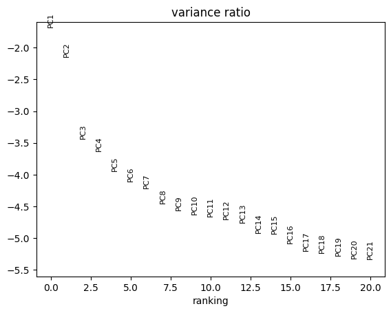
[13]:
sc.tl.pca(adata, svd_solver='arpack', use_highly_variable = True)

sc.pl.pca_variance_ratio(adata, log=True, n_pcs = 20) # visualize PCA variance explained
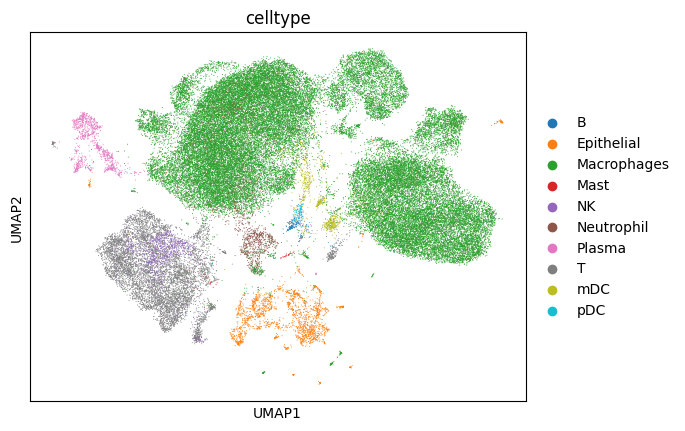
[14]:
sc.pp.neighbors(adata, n_neighbors=5, n_pcs=20)
sc.tl.umap(adata)

# plot pre-annotated cell types
sc.pl.umap(adata, color=['celltype'])
[15]:
adata
[15]:
AnnData object with n_obs × n_vars = 62551 × 24798
    obs: 'sample', 'sample_new', 'group', 'disease', 'hasnCoV', 'cluster', 'celltype', 'condition', 'n_genes_by_counts', 'total_counts', 'total_counts_mt', 'pct_counts_mt', 'n_genes'
    var: 'mt', 'n_cells_by_counts', 'mean_counts', 'pct_dropout_by_counts', 'total_counts', 'n_cells', 'highly_variable', 'means', 'dispersions', 'dispersions_norm', 'highly_variable_nbatches', 'highly_variable_intersection'
    uns: 'log1p', 'hvg', 'pca', 'neighbors', 'umap', 'celltype_colors'
    obsm: 'X_pca', 'X_umap'
    varm: 'PCs'
    layers: 'counts'
    obsp: 'distances', 'connectivities'
Save the data for downsteam analysis
[16]:
adata.write_h5ad(os.path.join(data_path, 'processed.h5ad'), compression='gzip')